STIN300 - Day 3 - Homework
Lars Snipen • Jon Olav Vik
1 The hexadecimal number system
Below we will look closer at colors. To do this we need to know some basics about the hexadecimal number system.
This number system has sixteen as a base-number, unlike our usual decimal number system where ten is the base. The digits in the hexadecimal system are 0,1,2,3,4,5,6,7,8,9,A,B,C,D,E,F. The first ten characters are our usual digits, and A means ten, B means eleven,…, F means fifteen.
Our usual decimal number system is position-based, i.e. to write the value ten we use two digits, 10. Then we increase the last digit until we reach 19, and then we increase the first and start over again at 20. With two digits we can reach up to 99 (ninety-nine).
The same applies to the hexadecimal system, but we write digits up to fifteen instead of nine. The value fifteen is the digit F and sixteen is written 10. Then 11 means seventeen, 12, means eighteen,…, 1F means thirty-one and 20 means thirty-two. With two digits we can reach up to FF (two hundred and fifty-five).
Most people are so ‘brainwashed’ with the decimal number system that we have problems digesting this at first. But, realize that all position based number systems follow the same rules, but varies the base. Here is a mini-exercise:
- In the decimal number system (base ten) the number 10 is the value ten
- In the hexadecimal number system (base sixteen) the number 10 is the value ____
- In the binary number system (base 2) the number 10 is the value ___
2 Exercises
In the exercises below there is a button. Try first to make the code to solve the exercise, then press the Code button to see a suggested solution.
2.1 Exercise - the RGB-colors
Coloring is often important when plotting. We have seen that there are some named colors available in R. Get an overview of all such named colors by typing colors() in the Console (and return).
Colors are typically specified as a vector of 3 values in the Red-Green-Blue channel (RGB-colors). We can use the function rgb() to illustrate this. Open the code-chunk and have a look:
library(tidyverse)
gg <- ggplot(tibble(1))+
  geom_point(aes(x = 1, y = 1), size = 100,
             color = rgb(red = 0.5, green = 0.5, blue = 0.5))  # specify color by rgb()
print(gg)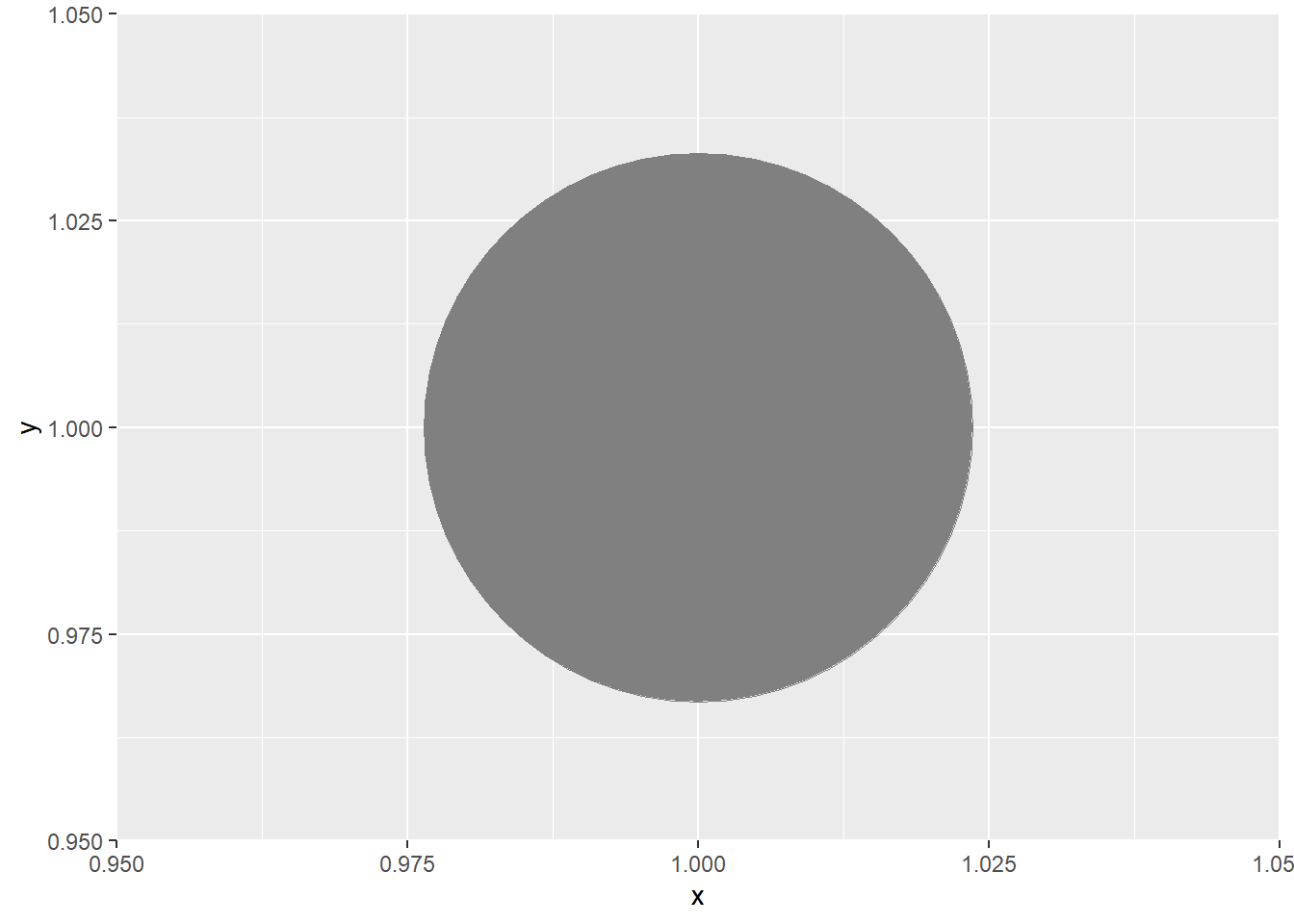
In rgb() we specify the level of red, green and blue in the mix, all of them being values between 0 and 1. Since all are 0.5 we get a gray color.
Now, change the red-, green- and blue-values between 0 and 1, and you get various colors. Try also the extremes, i.e. all are 0 or all are 1.
2.2 Exercise - colors as hexadecimal strings
Try to run the code x <- rgb(0.1, 0.2, 0.3). Inspect the object x. This is a color in R, displayed as a hexadecimal string.
This can be translated into a vector of three values! The first "#" just indicates this is a hexadecimal string. The last 6 characters are digits in the hexadecimal number system. Thus, a two-digit hexadecimal integer can take all values from zero ("00") up to two-hundred-and-fifty-five ("FF"). In the string above the first two digits indicate the red-value, the next two is the green-values and the last two is the blue-value.
What are the red-green-blue values in "#88A50F" if you translate it to our usual decimal numbers? Try to compute it manually first, then use the col2rgb() function to find the answer.
What is the hexadecimal strings for black and white? Try to compute it manually first, then use rgb() to find the answer.
print(col2rgb("#88A50F"))
print(rgb(0,0,0))
print(rgb(1,1,1))
2.3 Exercise - vector of colors
Earlier today we made a plot of some data from the mpg data set, and added manual colors. Instead of naming a set of 7 colors, use the rgb() function to create colors where green and blue are fixed at 0.5, and where red varies from 0 to 1, over 7 equally spaced values. HINT: Use the seq() function to create a vector of equally spaced values.
fig <- ggplot(mpg) +
  geom_point(mapping = aes(x = displ, y = hwy, color = class)) +
  scale_discrete_manual(aesthetic = "color",
                        values = rgb(seq(0,1,1/6), 0.5, 0.5))
print(fig)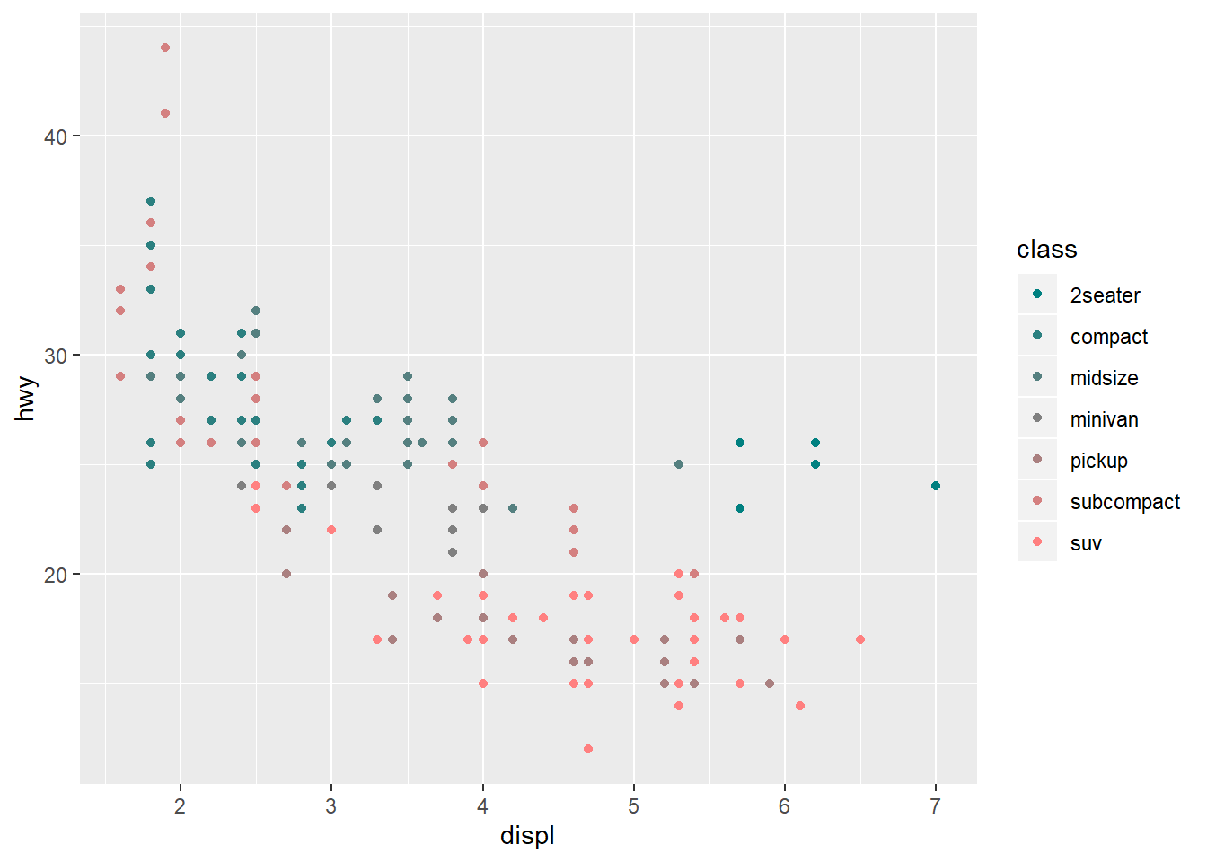
2.4 Exercise - color palettes
A color palette is a function that produces a set of colors given some input. Here is an example of a built-in palette: cols <- rainbow(8). The function rainbow() will produce a range of colors, and the input 8 means it creates eight different colors this time. These will be stored as a vector of colors in the object cols. We can now use this vector when we plot.
Different palettes produce different colors. We typically use palettes when we want the colors to change gradually, e.g. when mapping color to some continuous variable. Here is an example (open this code-chunk right away):
fig <- ggplot(mpg) +
  geom_point(mapping = aes(x = displ, y = hwy, color = cty))
print(fig)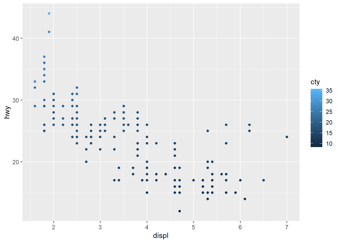
Notice how the colors indicate a continuous change, not a discrete change. The ggplot tends to interpret numeric variables as continuous. The column cty is numeric, hence, colors vary gradually according to some palette, here from black to blue.
Make the same plot as above, but use the rainbow() palette instead. Hint: Add a layer of scale by scale_color_gradientn(), and use rainbow() to specify its colours.
fig <- ggplot(mpg) +
  geom_point(mapping = aes(x = displ, y = hwy, color = cty)) +
  scale_color_gradientn(colors = rainbow(10))
print(fig)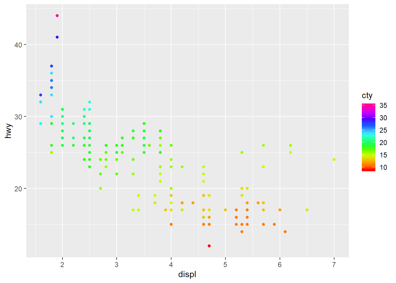
Here we used the scaling function scale_color_gradientn(), but there are other relatives of this function described in the same Help-file.
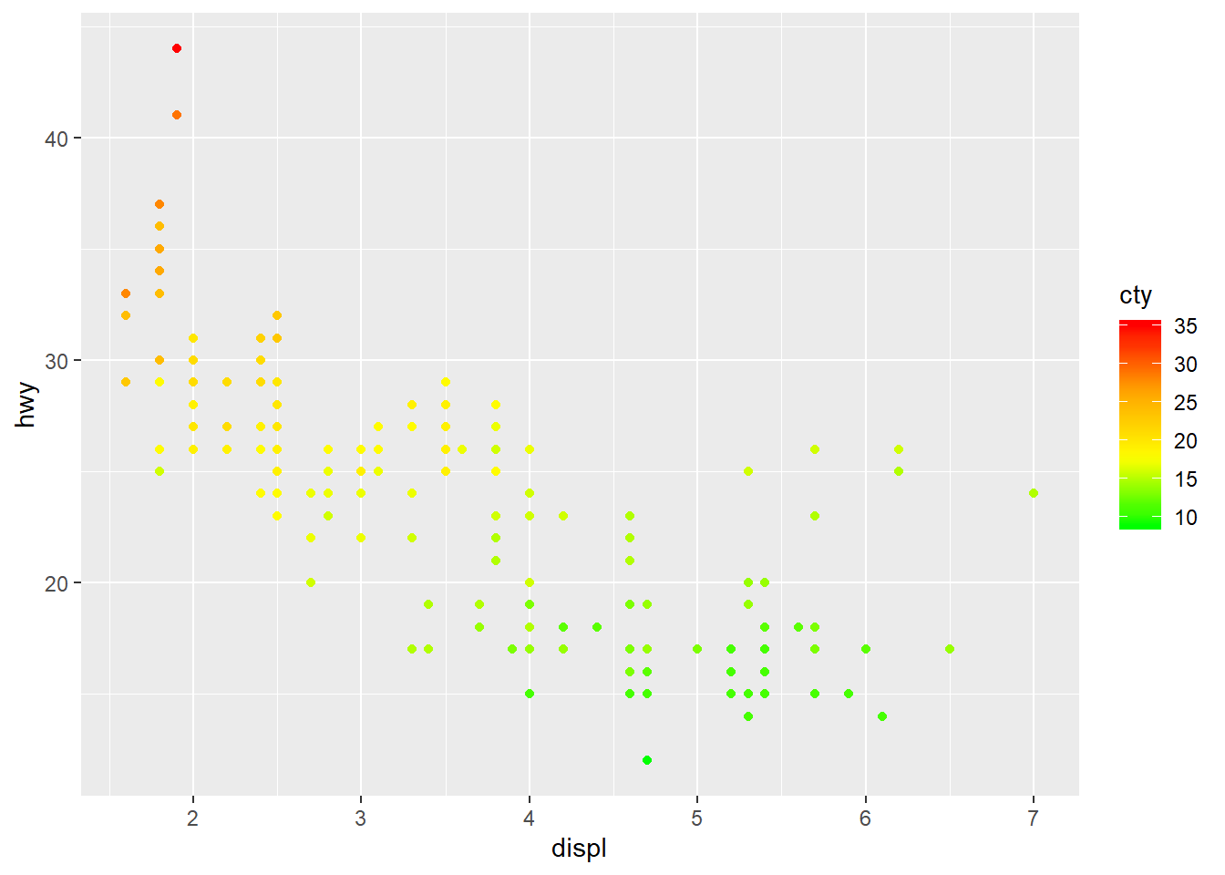
2.5 Exercise - making your own palette
You can easily create your own palette function! Let us replace rainbow() by a function that interpolates between the colors green-yellow-orange-red. We use the function colorRampPalette() to make the palette, i.e. this function builds another function! The function colorRampPalette should be given a vector of named colors green-yellow-orange-red, and will construct a function that interpolates between these. Store the result in my.palette. Thus, my.palette is now a function, not an object.
Next, replace the use of rainbow() above with your palette.
my.palette <- colorRampPalette(c("green", "yellow", "orange", "red"))
fig <- ggplot(mpg) +
  geom_point(mapping = aes(x = displ, y = hwy, color = cty)) +
  scale_color_gradientn(colors = my.palette(10))
print(fig)