STIN300 - Day 1
Lars Snipen • Jon Olav Vik
1 Today’s learning goals
The hyperlinks point to reference literature.
- Get started with R and RStudio. HOPR: Installing R and RStudio, The very basics
- Make R scripts, edit them and run R code. (HOPR)
- Basic knowledge of R data types. (HOPR)
- Basic knowledge of vectors.
- How to use some operators.
- Learn how to install R packages. (HOPR)
2 Getting started
This first part is not about programming, but to get the tools needed, and some first insight in how to use them.
2.1 Install R and RStudio
Follow these instructions.
2.1.1 ÆØÅ trouble on Mac?
Some Mac users experience this error message at startup:
Setting LC_CTYPE failed, using "C"…
They also experience R printing strange characters instead of æøå. Many have been helped by this witchcraft:
In the RStudio Console (where the > prompt awaits
your command), run
system("defaults write org.R-project.R force.LANG en_US.UTF-8")
Restart RStudio, and hopefully the error message will be gone.
2.2 Files and folders
Whenever we run R on our computer, it runs inside a folder (=directory). We refer to this as the working directory. We can easily change this during an R session, as we will see later. Anyway, all files and folders are always located relative to this Working Directory in R. Thus, we need to be aware of this Working Directory.
All computers, regardless of operating system, have a file tree, where all files and folders are organized in a hierarchy. On modern laptops the file tree is hidden behind a graphical display and you may not have any idea of where files are actually located. When we start using a computer for computing we need this insight.
2.3 Exercise - make a STIN300 folder for this course
Make a new folder named STIN300 on your computer that
you will use as the default working directory for R during this course.
You can in principle make this folder anywhere you like, but make
certain you know exactly where it is in the file tree! For convenience
it is a good idea to put it fairly close to the top if your file tree.
Regarding names of folders and files, there are some ‘rules’ that we
should always keep in mind:
- Never ever make folder names with spaces inside, like
STIN 300. Add an underscore if you want to separate words in the name (e.g.STIN_300). - Never use the non-English letters like æ, ø and å.
Most computers will allow you to make such names, but it is a hassle once we start programming. The exact same rules also apply when creating objects in R.
2.4 RStudio basics
Start RStudio. In this course we will not devote much time to the software RStudio as such, but we will pick up some insight as we go along. RStudio is our workplace when working with R, and we need some minimum insight. The RStudio workplace is split into \(2\times 2\) panes. Below is an example of how it looks when I am creating this document (which is R Markdown produced in RStudio).
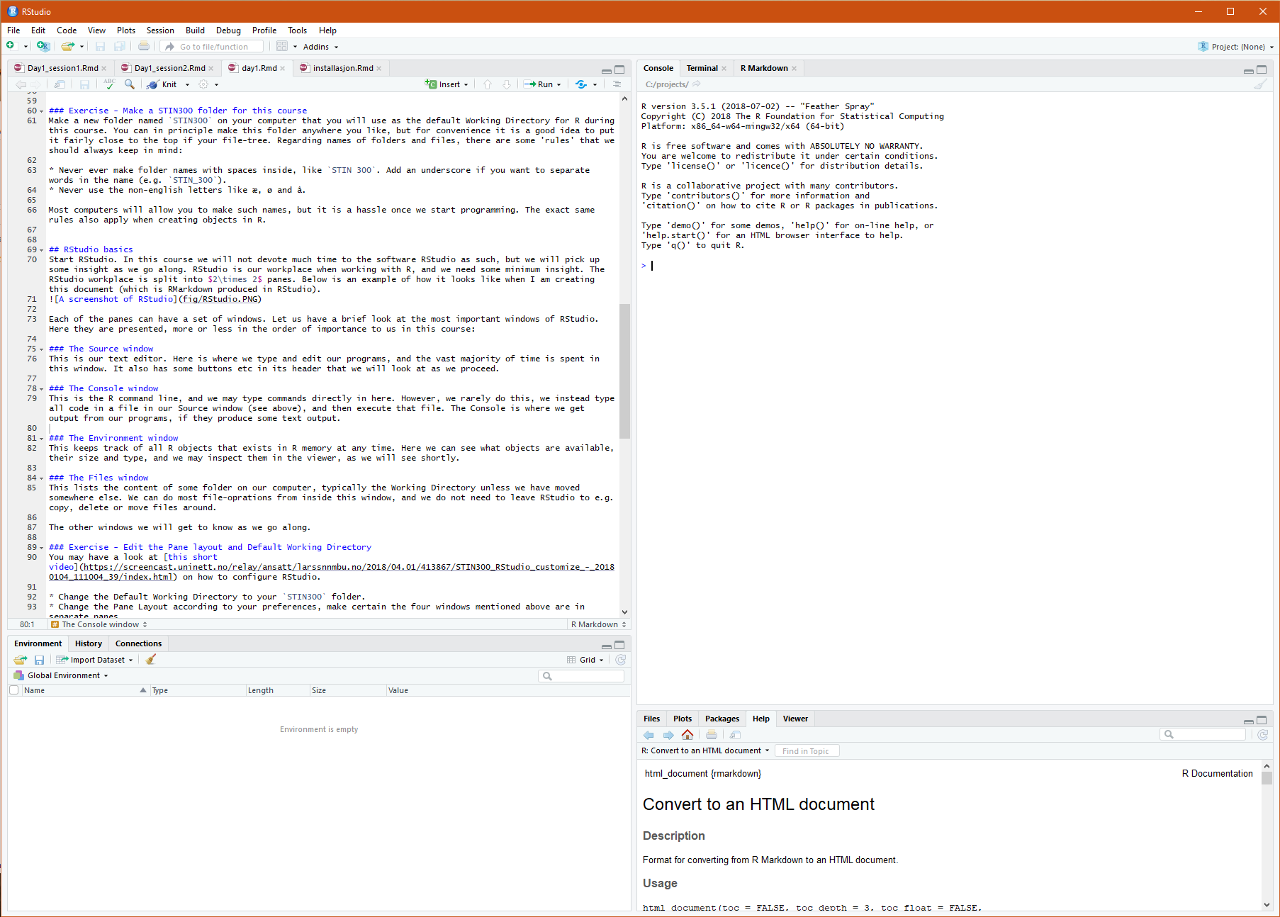
Each of the panes can have a set of windows. Let us have a brief look at the most important windows of RStudio. Here they are presented, more or less in the order of importance to us in this course:
2.4.1 The Source window
This is our text editor. Here is where we type and edit our programs, and the vast majority of time is spent in this window. It also has some buttons etc in its header that we will look at as we proceed.
Make yourself a document where you can take free-text
notes: File > New File > Text file. Here you
can take notes from the rest of this lesson.
2.4.2 The Console window
This is the R command line, and we may type commands directly in here. However, we rarely do this, we instead type all code in a file in our Source window (see above), and then execute that file. The Console is where we get output from our programs, if they produce some text output.
2.4.3 The Environment window
This keeps track of all R objects that exists in R memory at any time. Here we can see what objects are available, their size and type, and we may inspect them in the viewer, as we will see shortly.
2.4.4 The Files window
This lists the content of some folder on our computer, typically the Working Directory unless we have moved somewhere else. We can do most file operations from inside this window, and we do not need to leave RStudio to copy, delete or move files around.
The other windows we will get to know as we go along.
2.5 Exercise - edit the Pane layout and Default Working Directory
You may have a look at this short video on how to configure RStudio.
- Change the Default Working Directory to your
STIN300folder. - Change the Pane Layout according to your preferences, make certain the four windows mentioned above are in separate panes
After this, quit RStudio and re-start. In the header of the
Console window is listed the current Working Directory.
Verify this is according to your settings. Push the ‘arrow’ in the
header of the Console window, and you should be taken to the
File-window, displaying the content of this folder.
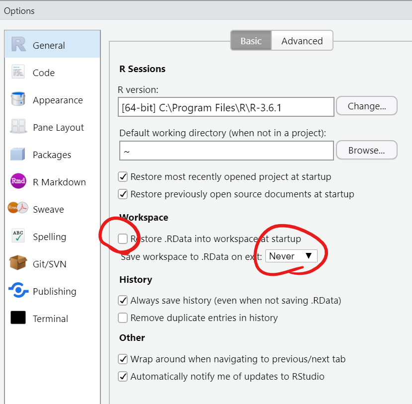
2.6 Exercise - modify some RStudio options to avoid a few pitfalls
If you just want to get going, follow the menu choices below and make sure the red-marked settings are as shown. Explanation follows below for those interested.
2.7 Tools > Global options…
Explanation:
Do not save/load .RData. R and RStudio offer to save
your variables to a file called .RData when you exit R, and
load them again the next time you start R. This is usually more
confusing than helpful. (If you wish to save the result of
time-consuming computations, you should do it yourself using
e.g. save().)
- The Environment pane gets crowded and unwieldy if all old variables accumulate there.
- If you create variables with the same name as R functions you need later, you may get confusing errors that only you experience.
- If you create a big dataset by accident, RStudio can take a long time to start/end due to the automatic loading and saving.
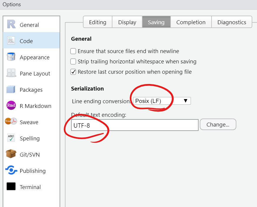
Use the same newline character on Windows as on Mac og Linux. Historically, these operating systems encoded line breaks in three different ways. R, however, is cross-platform, and it’s nice to have things behave the same.
Use the international character set UTF-8 in all text files. This ensures that æøå displays correctly, and also other scripts such as ひらがな og 漢字.
3 Some important phrases
Before we actually start programming, there are some words and phrases that need some explanation. These are data structures, data types and operators. Here is a short guide to what they mean:
3.1 Data types
This is the type of data we are handling. We need to distinguish between data types for several reasons. Some operations are only valid for numbers, some only for texts, etc. Below we list the three basic data types we meet right away when we start R programming.
3.1.1 Numbers
In most cases we handle data as numbers. In R we meet two data types
for numbers. The first is numeric, and all decimal numbers
are of this type, e.g 3.14. This is also sometimes referred
to as a double (dbl). The other data type for
numbers is integer, e.g. 10. R is not fussy
about the distinction between numeric and
integer, and we will not be either. Think of them both as
numbers!
3.1.2 Text, also known as “strings” or “characters”
The next common data type is character. All
texts are of type character.
3.1.3 Logicals
The third common data type is logical. This can only
take two values, either TRUE or FALSE. This
data type is found in all programming languages, and we will see them a
lot. If we make some kind of comparison in our programs, the
result of this is always a logical.
There are other data types in R, we will see some of them later.
3.2 Data structures
A data structure is simply the way data are organized in R memory. We will later today see the most common data structures in R, a vector.
Data stored in a vector are simply lined up after each other, as in a series. This is a very basic data structure. It is also referred to as an array, but in R we denote it a vector. We will see other data structures later, e.g. tables and lists.
3.3 Operators
Operators are symbols with special meaning, e.g. the sign
+ means ‘plus’, and is used to add two numbers (either
numeric or integer). We will meet the first
operators today, but more will be encountered over the next three
weeks.
4 First programs
Time to start using R!
4.1 Scripting and R objects
Let us immediately make an R script where we have two R objects storing the height and the radius of some cylinder. Using these values, the code should then compute the volume of the cylinder, and print out the answer. Here is the ‘answer’:
height <- 15  # height in cm
radius <- 3   # radius in cm
volume <- pi * radius^2 * height
volume
## [1] 424.115Notice that R automatically prints the value of an expression that is not assigned to a variable. This is called “implicit printing”. (Implicit printing does not happen within functions or loops.)
Here is a short video that takes you through this, and where we also look at some RStudio basics as we go along.
Let us reflect upon what we did. An R script is simply a text file
with R code in it. It should always end with the extension
.R. When we execute, or source, a script, the
code-lines are executed from the top down, one by one. Actually, we
could have copied them into the Console window and executed them one by
one and got the exact same result. The idea of having it in a script is
of course that we can re-run the code any time, and we can easily edit
it. Commands executed in the Console are not stored (well, if you
inspect the History window you will see this is not entirely
TRUE…;)
We create R objects simply by naming them and assign some
value to them. The assignment operator in R is the ‘arrow’
<-. You can also use the =, but there is a
convention of using the arrow. The = operator is used for
assigning values to function arguments, as we will see later. What is an
R object? Think of it as a location in the computer memory where some
data has been stored. The location has a name, it stores some data type
and it has some value. All programming is about creating and
manipulating such objects! In the Environment window we see all this
listed (select Grid view instead of List view in the window header).
Notice the comment symbol #. Everything we write
after the # is not interpreted by R, and
we may write anything we want. We use this to add comments to our
code.
When we are building programs, we do it step-by-step. Make it a habit to follow this procedure:
- Add some comments about what to do, and possibly how to do it.
- Add a small amount of code.
- Save the script file!
- Source (run) the code, and see if it works.
- If not, try to correct the error.
- When everything looks fine, return to the top, and add more code.
Let us extend the previous exercise…
4.2 Exercise - more cylinders
Add an R object containing the text "Cylinder volume ="
and print the result, using the command cat():
height <- 15  # height in cm
radius <- 3   # radius in cm
volume <- pi * radius^2 * height
txt <- "Cylinder volume ="
cat(txt, volume, "\n")
HINT: To find help on the command cat(), try to google
with this search-phrase:
stackoverflow how to use cat in R
Actually, the website Stack Overflow is a goldmine for learning R (and most other programming languages).
Here is another short video on how we can solve this.
4.3 Reassignment
Before we end our first scripting, just a word of caution. In R we can re-assign values and data type to existing objects at any time, and this does not produce any warning or error. Here is a short code that demonstrates this:
height <- 15  # height in cm
radius <- 3   # radius in cm
#...many lines of code here...
height <- "large"
Run this code line-by-line (use the Run-button).
The object height first contains a number, but then it
is re-assigned to contain a text. If you proceed trying to compute the
volume, assuming height is numerical, the program crashes.
How can we guard against this? First, using good object names, not silly
names like x and y, but meaningful names,
makes it less probable you accidentally re-use object names. Next,
instead of having huge scripts, we build functions, which we
will talk more about later. In functions we can re-use names used in
other functions without problems.
5 Vectors
The vector is the most basic data structure in R. In fact, we have already used it! The R objects we created above were all vectors.
A vector is a linear structure of data. Above we created a vector
named height and filled it with 1 value. That is OK, but a
vector we can have as many values as our computer memory allows. We can
draw an image of a vector like this:
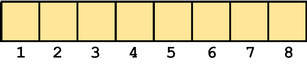
There is one fundamental rule for vector in R: In a vector there can only be data of one data type. In the figure above this is indicated by all cells having the same color.
This means that all elements in the vector must be of the same type, i.e. either all are numbers, all are texts, etc. If you want to mix data of different types, you must use a list, which we will talk about later. Since vectors have this restriction, they are extremely fast to operate on. If speed is important, try to keep data in vectors.
5.1 Creating vectors
Here are some basic ways of creating vectors that we make use of from time to time
- Manually type in values:
names <- c("Lars", "Jon Olav", "Torgeir"). Notice we writec()and inside the parentheses we list the elements separated by commas. - Series of integers:
numbers <- 1:10. The R objectnumbersbecomes a vector with the numbers 1,2,…,10. - Sequence of any kind:
heights <- seq(from = 0.1, to = 100, by = 0.1). Type?seqin the Console window, and read the Help-file forseq(). All R functions (commands) have a Help-file that you find by typing?followed by the function name, in the Console.
We will see more ways to create vectors later. The command
c() is what we also use if we want to combine two
already existing vectors into one new, e.g. we could have written
c(numbers, heights) and ‘glued’ the vectors
numbers and heights into one long vector. Note
that this is fine since both vectors contain numbers, remember: a vector
can only contain one single data type. You can never combine a vector
with numbers and a vector with texts into a single vector (without
something being destroyed/changed).
5.2 Special characters
R and R Markdown (which we’ll see shortly) use several symbols that you may never have used before. Check that you know how to type all of the following:
[]square brackets, used to index vectors, e.g.x[10]and to specify R Markdown chunk options.{}curly brackets, used to group multiple statements, e.g. in loops and functions, see day 8.`backtick:- Single backticks allow you to use “non-syntactic” variable names:
`fancy variable` <- 42 - Single backticks in R Markdown marks text as
code. - Triple backticks in R Markdown delineates a code chunk.
- Single backticks allow you to use “non-syntactic” variable names:
^the caret, used for exponentiation:2^5.~the tilde, used to specify statistical models, e.g.y ~ x, to denote your “home directory” on Mac and Linux, and for various Tidyverse black magic.$dollar sign, used for indexing list elements and object attributes.#hash sign, used for comments in R code and headings in R Markdown.\backslash: used in strings to write some special characters such as the tab\tand the newline\n. To put an actual backslash in a string, “escape” it with another backslash:cat("\\").F1: if your cursor is inside a word in R code, F1 will bring up Help on that word.
On many laptops, the F1 key also has other uses, such as turning sound on/off or putting the computer to sleep. In that case, there is often anFnkey that toggles what the key should do.|: Logical OR operator.
How you type these depends on your operating system (Windows/Mac/Linux) and keyboard layout.
Here are my notes; please email jon.vik@nmbu.no about anything missing:
Norwegian Windows:
{[]}areAltGr + 7890.- Backtick is a “dead key”: Nothing is shown until you type a
character it applies to (in our case, a Space).
- While holding
Shift, press and release the key to the right of the plus sign. - Release
Shiftand pressSpace. (Or a vowel to get a grave accent, e.g. à.)
- While holding
- The caret works the same, but with the key to the right of Å.
- The tilde is similar, but different:
- While holding
AltGr, press and release the key to the right of the plus sign. - Release
AltGrand pressSpace. (Or “n” if you want to type ñ, etc.)
- While holding
Norwegian Mac:
- Caret
^isShift + ˆfollowed by Enter. (The tiny caret-like symbol is called a combining circumflex accent, I think.) [is Option + 8.|is Option + 7.
5.3 Indexing
The brackets [ and ] have a special meaning
in R: They are used to index or subset some data structure, which means
we select a subset of the data in some data structure.
Assume we want to do something to element number 3 in a vector named
heights. Could be we would like to copy that value to some
other R object, or perhaps change that value. By using the notation
heights[3] we refer to element number 3 in the
vector named heights. Note: It is not the element
whose value is 3, it is element number 3, counted from the start, see
Figure 2 above. The first element in a vector is element number 1 (and
not number 0 as in some other languages).
We can index many elements in a go, e.g. if we write
heights[1:5] it means we refer to the vector consisting of
elements 1 up to 5 in heights.
5.4 Exercise - indexing a vector
Create a vector x consisting of the integers from 10 to
20. Copy elements number 2 to 4 from x to a new vector
named y. Copy elements 10 to 15 from x to
another new vector z. Copy and fill in the gaps:
x <- ____
y <- ____
__ <- x[____]
Source the code, and inspect all three vectors. What happens, and why?
Well, here you should see the value NA for the first
time. It is short for Not Available, and indicates elements without
content. We will see NAs quite often in R, mot typically if
we read in a table of data, and there are cells without content. These
will typically be filled with a NA. Think of it as
missing data.
The reason we see NAs above is that we try to access
elements who are not there. There are no elements number 12, 13, 14 and
15 in x, it has only 11 elements. Unlike some other
programming languages, R does not give you an error here, but fills
z with NAs.
5.5 Length and names
How can we find the length of a vector?
The length is simply the number of elements in the vector, and of
course we can see that in the Environment. But, what if we want to use
this in our code somewhere? Then we use length():
x <- 5:1
n <- length(x)    # number of elements in x
If we want to copy the last element in x, we need to
know its length, and then index with this. For those familiar with
Python, the following example is extra important:
a <- x[length(x)]   # what is copied here?
b <- x[-1]          # what is copied here?
Have a look at the result, and learn.
Each element in a vector may have a name! This means we add a (short) text as a ‘tag’ to each element:
named.vector <- c(Monday = 1, Tuesday = 2, Friday = 5)Note that the vector is numeric because the actual
content are numbers (1,2, and 5). The names are not part of the vector
itself, they are just some additional information.
You can use the function names() to both give names to
or copy names from a named vectors, read its Help-file by typing
?names in the Console.
5.6 Exercise - more vectors
Make a vector weekdays containing the weekdays (Monday,
Tuesday, etc.). Make another R object called weekend, and
copy the weekend days to this. Reverse the order of the elements in
weekdays. Hint: Create a vector of integers from 7 to 1,
and use this to index. Copy, and fill in the gaps
weekdays <- __"Monday","Tuesday","Wednesday","Thursday","Friday","Saturday","Sunday"__
weekend <- weekdays[____]
index.vector <- ____
week.reversed <- ____
6 Basic operators
6.1 Arithmetic operators
We have already seen some basic arithmetic operators in use above: multiplication and power. Here they are all listed:
- Plus
x + y - Minus
x - y - Multiplication
x * y - Division
x / y - Power
x^y
Note: the blank around the operators (except the last one) are not required, but it is a convention in R. In general, R is very liberal with spaces in the code. Learn more about code-conventions in the homework exercises.
6.2 Relational operators
In R we also have all the common relational operators that we use to compare objects:
- Smaller than
x < y - Larger than
x > y - Smaller than or equal
x <= y - Larger than or equal
x >= y - Equality
x == y - Not equal
x != y
Note the huge difference between x == y and
x = y! The first is a comparison, we test if the
content of x and y is identical. The outcome
of this is either TRUE or FALSE. The latter is
a assignment, where we copy the value(s) of
y into the object x. This is the same as
x <- y, and is one reason why we always recommend using
the arrow <- as the assignment operator. It is a very
common mistake to use == instead of = or vice
versa!
Comparisons are typically used for data of either type
numeric or integer, but they also work for
texts! Try out "a" < "b" etc. to see how these operators
work for texts.
All comparisons produce a logical as a result,
regardless of what is compared. This is how data of type
logical are being produced, we rarely create them
explicitly.
6.3 Exercise - operator precedence
Operators have the same precedence in R as in any other software that do calculations. First, compute manually what the result should be here, and see if it matches what R gives you:
result <- 1 + 2 * 3 - 4^2 / 26.4 Vectorized code
What is somewhat special to R is that operators typically work elementwise. What does it mean?
Let us make two vectors: x <- c(2, 3, 5) and
y <- c(1, 1, 1). Both have 3 elements. We can add them,
like this: z <- x + y, just as if they were single
numbers. The resulting vector z also has 3 elements, and we
can see that the first element of x was added to the first
element of y to produce the first element of
z, and so on. This makes R code extremely short and very
fast!
The fact that we can operate on entire vectors like this is a huge asset to R, and it is important that you learn to make use of it. It is referred to as vectorized code.
6.5 Exercise - reverse vector
Create a vector x with the integers from 1 to 10.
Subtract 11 from all elements in x, and then multiply all
elements by -1. Store the result in y.
x <- ____
y <- (____) * ____
Notice the data types of x and y.
6.6 Recycling
What we saw in the above exercise is what is known as recycling in R. It is important to understand this, both because we make use of it, but also because it may cause some errors if you are not aware of it.
In order to use operators on two vectors, the vectors should in principle be of the same length, i.e have exactly the same number of elements. However, if you try to operate on two vectors of different lengths, R will in many cases (but not always) re-cycle the shorter one to make it the same length as the longer, and then perform the operation.
This is what we saw above: We tried to subtract a vector of 1 element
(11) from a vector of 10 elements (x). This
should not really be possible, but behind the scene R will copy the
shorter vector 10 times, and then we can do the elementwise
subtractions. This is not exactly how it is done, but it is how we
should think of it! Anyway, we end up with a vector having the same
number of elements as the longest. Notice that we were not warned about
this!
Now, try to change the code slightly, replace x - 11
with x - c(11, 11, 11). Re-run this and see what
happens.
6.7 Exercise - beer can design
We want to produce an ecological beer can, using as little aluminium as possible. Each beer can must have a cylindrical shape, and the volume of the beer can must always be 0.5 litres (\(500 cm^3\)). The amount of aluminium used is proportional to the surface area of the beer can, i.e. we want a beer can with as little surface area as possible, but still under the restriction that it must contain \(500cm^3\).
Make a script where you give a value to the can height (in cm), and then computes the radius of the cylinder from the volume-restriction. The formula for the volume of a cylinder is \(V=\pi r^2 h\) where \(r\) is the radius and \(h\) is the height. This means \(r=\sqrt{V/(\pi h)}\), and since the volume is always \(V=500\) you compute the radius for any given height.
Then you compute the surface-area of the corresponding beer can. The formula for the surface area of a cylinder is \(A = 2\pi r^2 + 2\pi rh\) where \(r\) is the radius and \(h\) is the height.
The constant \(\pi\) is already
defined and is named pi in R.
Make a vector of different heights, and compute a vector of areas.
Find approximately the optimal ecological beer can height by
first using the function which.min() on the computed areas,
and then use this result to print the optimal height.
volume <- 500
height <- seq(from=1, to=30, by=0.1)
radius <- (volume / (pi * height))^(0.5)
area <- 2 * pi * radius^2 + 2 * pi * radius * height
cat("Optimal height is", height[which.min(area)], "\n")
7 R packages
A main idea in R is that code for different purposes are grouped into packages that you may or may not install. When you install R you get a set of base packages that contain some basic functionality that we all need. All we have seen so far are in these packages. This makes the basic R installation comparatively small.
In addition to the base-packages there is a plethora of other R-packages that you may install. Each package typically contains a collection of functions and data related to some topic. Some packages are huge, but most are smallish, containing a few functions. Many packages depend on other packages, and in order to make it work you need to install all the dependencies as well. The main repository for such packages is CRAN, the Comprehensive R Archive Network. They maintain a database of R packages satisfying certain quality requirements.
7.1 Installing R packages
From RStudio it is very simple to install R packages, and here is a short video on how to.
You typically install a package once, but you may need to update it from time to time. Under the Tools-menu in RStudio you find a Check for Package Updates…
7.2 Loading R packages
In order to start using it, the package must be loaded. This
is done by the library() command, e.g. if you have
installed the package MASS, you load it by having
library(MASS) in your code. This must be done once
every R session, and for this reason it is a good habit to place
such library() statements at the top of each script where
the package is used. It doesn’t matter if you load it more than
once.
Remember:
- We install a package once
- We load the package each time we use it
7.3 Exercise - install tidyverse
Packages can be bundled together into larger collections, and the
tidyverse is an example of this, containing several
packages sharing a common coding-philosophy. Instead of installing all
these packages one by one we install tidyverse as if it was
one package.
- Install the
tidyverse-packages on your computer.
There will typically be a lot of output in the Console during
installation. If it succeeds, you should be able to load the package by
typing library(tidyverse) in the Console window.
Tomorrow we will start using the tidyverse packages.
8 R Markdown
R Markdown lets us write reports mixing explanatory text, R code and output such as tables and figures. The generation of the report from the Rmd source document is called knitting. It helps make your research reproducible: You can modify and refine your Rmd document, then easily re-knit. This also makes it easy for collaborators, supervisors or teachers to suggest fixes or refinements to your work.
8.1 Exercise - Knit the sample R Markdown document
RStudio > File > New File > R Markdown…, press OK and click the Knit button.
After a few seconds, an HTML report pops up in the RStudio Viewer pane. Once you’ve admired the report, look at the sample Rmd file in more detail to see the codes that specify headings, etc.