Indices and tables
Assessing line quality using the BOS method
The BOS Plugin compares the geometries of two line layers (the input layer X and the reference layer Q) by buffering and overlay for several buffer sizes, collecting statistics and plotting the results for a visual assessment of the quality (geometric accuracy, bias, completeness and miscodings) of the input line data set with respect to the reference line data set according to the BOS method [Tveite1999].
The Buffer-Overlay-Statistics (BOS) method
The Buffer-Overlay-Statistics (BOS) method works on line data sets and produces graphs that indicate spatial accuracy, bias, completeness and miscodings for a line data set of unknown quality with respect to a data set of better quality.
The core of the method is buffering around the lines of the two data sets using a number of buffer sizes, and combining the resulting buffer data sets (XB and QB) and the two input line data sets (X and Q) in various ways to produce statistics that can be plotted to reveal the characteristics of the input line data set, X, with respect to the reference data set, Q.
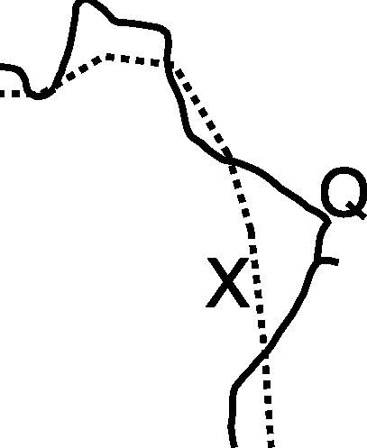
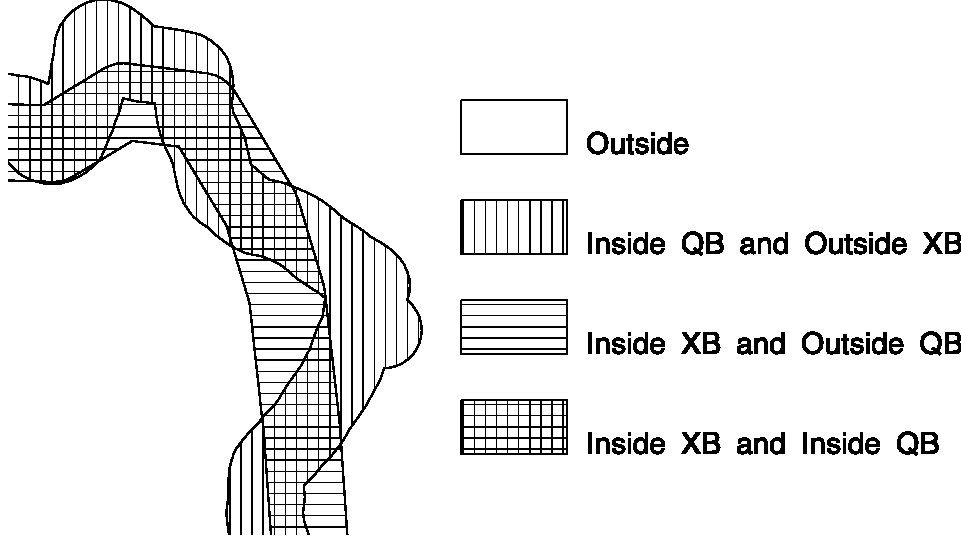
The basic elements of the BOS method are illustrated below.
The elements of the BOS method |
|
|---|---|
Line data sets (X and Q) |
Buffer (XB, QB) combination |
For each of the chosen buffer sizes, buffers are created and combined using an overlay operation to produce the polygon layer illustrated in the right part of the above illustration.
Output
Four types of graphs are produced, and the type of graph to be shown is selected using the Graph combo box / menu. The following graphs are offered:
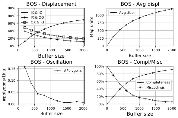
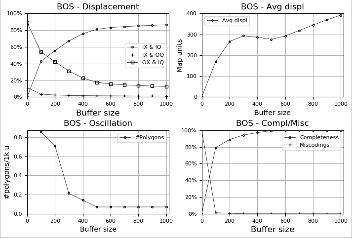
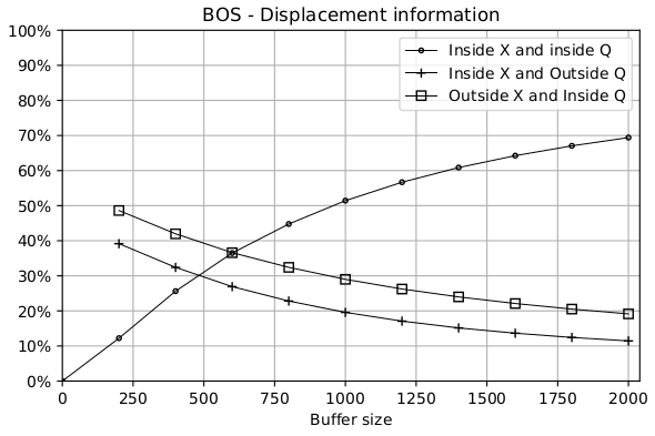
Displacement - Shows normalised (0%-100%) relative area sums for the polygons in the combined buffer data set, grouped according to the following combinations Inside X and Inside Q, Inside X and Outside Q, Outside X and Inside Q.
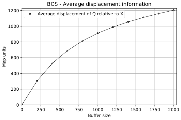
Average displacement - shows the average displacement as a function of buffer radius. Is expected to flatten out when the average displacement is equal to the spatial accuracy.
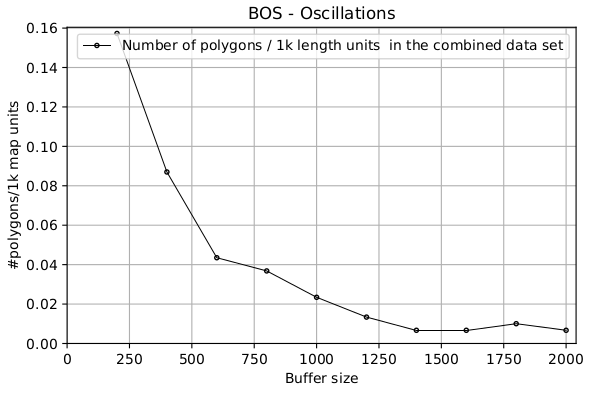
Oscillations - can indicate bias and spatial accuracy. If the graph is not steadily decreasing, it can be taken as an indication of bias.
Completeness / Miscodings - shows completeness and miscodings (two graphs in the same plot) as a function of buffer radius.
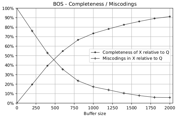
In addition a combination of all the graphs is offered with the “Combined” option.
Options
The behaviour of the BOS plugin is configured in the GUI:
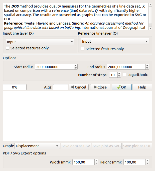
For input layers, you can choose if Selected features only are to be considered.
In the Options area you will find the following:
The Number of steps (buffer sizes) - minimum 2
The Start radius (for the buffers)
The End radius (for the buffers)
It is possible to choose a Logarithmic distribution of the buffer sizes. The default is to distribute them evenly between the Start radius and End radius.
If you would like to have 10 buffers with a spacing of 100, you could specify 100 for the Start radius, 1000 for the End radius and 10 for the Number of steps, resulting in the following buffer sizes:
100, 200, 300, 400, 500, 600, 700, 800, 900, 1000
With Start radius 1, End radius 1000, 10 buffers and Logaritmic the list will be:
1, 2.15, 4.6, 10, 21.5, 46.4, 100, 215.4, 464.2, 1000
Depending on your datasets, it may be useful to start with a small radius, for instance a Start radius of 1 with an End radius of 1000. The steps will then not be at “nice” numbers, but the first data point will be close to the start of the x (buffer size) axis. The Logaritmic option is useful in combination with a small start radius, in order to get more details in what is normally the most “interesting” range.
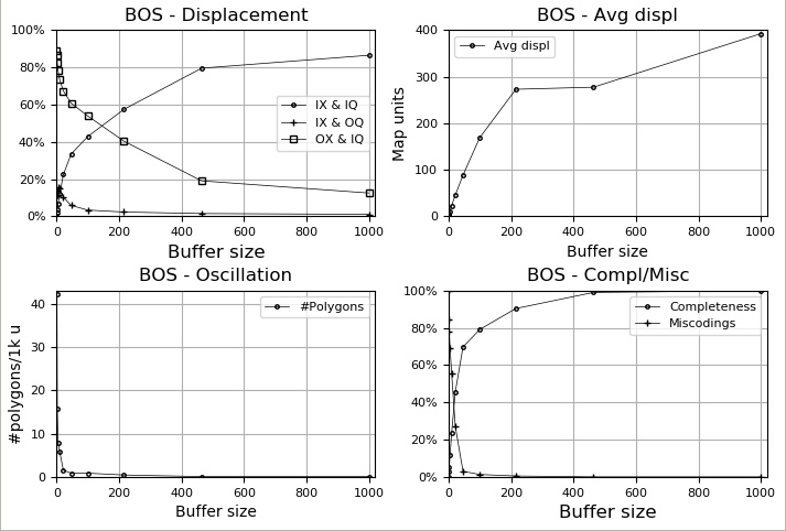
The plots in the figure below show the effect of the Logarithmic option (Number of steps: 10; Start radius: 10 for linear and 1 for Logarithmic; End radius: 100).
Linear |
Logarithmic |
|---|---|
Output options
When the algorithm has run, you can choose the type of graph (see descriptions above). Choices are:
Displacement
Average displacement
Oscillations
Completeness
Combined - all the four graphs listed above are combined into one plot
Export
Export is supported for plots and data.
Exporting plots as PDF and SVG
Export of plots is supported with the buttons Save plot as SVG and Save plot as PDF.
Options:
Width (mm) - The width of the output graphics in mm. Default: 150.0 mm
Height (mm) - The height of the output graphics in mm. Default: 100.0 mm
Exporting the data as CSV
The statistics data can be exported to CSV for further processing or tailored visualisation. The first (header) row contains identifiers / names for the columns. The exported CSV consists of nine columns, and as many rows as there are steps (plus the header row). The CSV-file looks like this (five steps in this example):
radius;IR;I;R;O;completeness;miscodings;average_displacement;oscillations
200.0;28500509.552210856;91345651.61111134;113376990.93457934;6068139105.312706;0.19671702510313907;0.7601548286200464;594.4025546563738;0.1974226191819506
400.0;106114289.65340048;134189530.21981135;173808986.21196535;5890899886.840816;0.3941682281114015;0.5284117923479394;908.9111184324876;0.11376896698620881
600.0;207985731.5163426;153389969.1893688;208527378.02795056;5740443047.301017;0.5479680819839098;0.3559997748555806;1087.6903083504928;0.06692292175659341
800.0;320066918.213234;162997040.60599986;231709138.4748819;5602226235.222582;0.6662973341813202;0.23494762857415086;1205.5310091551798;0.06023062958093407
1000.0;438372775.45679665;166790573.15283233;247128084.98095602;5472587533.011159;0.7345931607936302;0.17208001554203864;1282.9193606248948;0.04349989914178572
A CSVT file (with the same prefix as the CSV file, but a csvt
suffix) specifying the data types of the columns is also created,
with the following content:
"String", "Real", "Real", "Real", "Real", "Real", "Real", "Real", "Real", "Real", "Real"
Warning
The method involves a lot of computation and will therefore take a very long time for data sets that are not extremely small. The running time will increase with the number of steps.
Implementation
The heavy work is performed in the background using a worker thread. Most of the computation is performed in the worker thread using QGIS processing algorithms (Buffer, Union, Clip, Difference, Multipart to singleparts and Statistics by categories).
The main (left) progress bar is updated each time a main step (buffer size) has been completed, and the second (right) progress bar reports the progress of the individual processing algorithms (there are eight substeps for each buffer size). The current algorithm/substep is indicated in the area between the progress bars: “prep”, “inpb (1/8)”, “refb (2/8)”, “clip (3/8)”, “diff (4/8)”, “union1 (5/8)”, “union2 (6/8)”, “tosingle (7/8)” and “stat (8/8)”.
Versions
The current version is 1.1.0.
- 1.1.0
Set the minimum number of steps to 2 (#1)
- 1.0.1
Eliminated the superfluous “BOS” submenu under the Vector menu
Documentation update
Code cleaning (PEP 8)
1.0: First official version.
Citation
Would you like to cite / reference this plugin?
Tveite, H. (2020). The QGIS BOS Plugin. <URL: http://plugins.qgis.org/plugins/BOS/>.
Bibtex:
@misc{tveitebos,
  author = {Håvard Tveite},
  title = {The {QGIS} {BOS} Plugin},
  howpublished = {\url{http://plugins.qgis.org/plugins/BOS/}},
  year = {2020}
}
References
- Tveite1999
Tveite, H. and Langaas S., 1999. An accuracy assessment method for geographical line data sets based on buffering. International Journal of Geographical Information Science, 13, pp. 27-47.
